After providing a baseline for Parallel Execution working as expected in the introduction of this series, in this part I’ll demonstrate how things can go wrong with the work distribution.
A Simple Example Of Parallel Execution Skew
One common source of Parallel Execution Skew is a skewed foreign key, which means that the value distribution of the foreign key column is skewed, with the majority of rows pointing to the same PK values of the parent table.
Following the description of parallel join processing from the previous part of this series, it becomes clear that in such a case a distribution based on the join key values will lead to a skewed work distribution – all rows having the same FK values will be processed by the same worker process, significantly influencing the overall execution time if these rows represent the majority of data volume to process.
For that purpose we’ll repeat the same query as in the previous article, but this time using the T_2.FK_ID_SKEW column in the join:
Serial execution:
|
1 2 3 4 5 6 7 8 9 10 11 12 13 14 15 16 17 |
select count(t_2_filler) from ( select /*+ monitor no_parallel leading(t_1 t_2) use_hash(t_2) no_swap_join_inputs(t_2) */ t_1.id as t_1_id , t_1.filler as t_1_filler , t_2.id as t_2_id , t_2.filler as t_2_filler from t_1 , t_2 where t_2.fk_id_skew = t_1.id and regexp_replace(t_2.filler, '^\s+([[:alnum:]]+)\s+$', lpad('\1', 10), 1, 1, 'c') >= regexp_replace(t_1.filler, '^\s+([[:alnum:]]+)\s+$', lpad('\1', 10), 1, 1, 'c') ); |
Parallel Execution:
|
1 2 3 4 5 6 7 8 9 10 11 12 13 14 15 16 17 |
select count(t_2_filler) from ( select /*+ monitor leading(t_1 t_2) use_hash(t_2) no_swap_join_inputs(t_2) pq_distribute(t_2 hash hash) */ t_1.id as t_1_id , t_1.filler as t_1_filler , t_2.id as t_2_id , t_2.filler as t_2_filler from t_1 , t_2 where t_2.fk_id_skew = t_1.id and regexp_replace(t_2.filler, '^\s+([[:alnum:]]+)\s+$', lpad('\1', 10), 1, 1, 'c') >= regexp_replace(t_1.filler, '^\s+([[:alnum:]]+)\s+$', lpad('\1', 10), 1, 1, 'c') ); |
The serial execution still takes approximately 57 seconds as before, but the Parallel Execution on my system takes approximately 45 seconds, which is faster than the serial one, but much slower than the 15 seconds of the “perfect” example demonstrated in the first part of this series.
I’ve made use of a simple CPU-intensive regular expression to make the problem more visible with a limited amount of data to process – of course this assumes that there is more than a single CPU available so that spreading the processing across multiple CPUs actually allows for getting the result quicker than with serial execution on a single CPU.
For simple parallel SQL executions that make use of data redistribution (most non-trivial SQL Parallel Execution requires data redistribution, only so called Full-Partition-Wise operations where the data is already partitioned in a suitable way can do parallel processing without data redistribution) the view V$PQ_TQSTAT can be used to gather information about the data distribution.
Note: The view V$PQ_TQSTAT is special because it is only populated in the private memory of the Query Coordinator session after successful completion of Parallel Execution. If the execution gets cancelled or encounters an error then the view won’t be populated. Since it is only populated in the Query Coordinator’s private memory you can’t query it from a different session. There are even more restrictions – for more complex Parallel Execution plans the view might return incorrect or even useless results, so it’s unfortunately not suitable for a generic troubleshooting procedure, but can be handy in simple cases like the one demonstrated here. For more information see the third part of my video tutorial “Analysing Parallel Execution Skew”.
Running the following query in the Query Coordinator’s session after completion of the statement we get the following result (use SQL*Plus to get the formatting shown):
|
1 2 3 4 5 6 7 8 9 10 11 12 13 14 15 16 17 18 19 20 21 22 23 24 25 26 27 28 29 30 31 32 33 34 35 36 37 38 39 40 41 42 43 44 45 46 47 48 49 50 51 |
break on dfo_number nodup on tq_id nodup on server_type skip 1 nodup on instance nodup select /*dfo_number , */tq_id , cast(server_type as varchar2(10)) as server_type , instance , cast(process as varchar2(8)) as process , num_rows , round(ratio_to_report(num_rows) over (partition by dfo_number, tq_id, server_type) * 100) as "%" , cast(rpad('#', round(num_rows * 10 / nullif(max(num_rows) over (partition by dfo_number, tq_id, server_type), 0)), '#') as varchar2(10)) as graph , round(bytes / 1024 / 1024) as mb , round(bytes / nullif(num_rows, 0)) as "bytes/row" from v$pq_tqstat order by dfo_number , tq_id , server_type desc , instance , process ; TQ_ID SERVER_TYP INSTANCE PROCESS NUM_ROWS % GRAPH MB bytes/row ---------- ---------- ---------- -------- ---------- ---------- ---------- ---------- ---------- 0 Producer 1 P004 493865 25 ########## 51 109 P005 508088 25 ########## 53 109 P006 504728 25 ########## 52 109 P007 493319 25 ########## 51 109 Consumer 1 P000 500363 25 ########## 52 109 P001 500256 25 ########## 52 109 P002 499609 25 ########## 52 109 P003 499772 25 ########## 52 109 1 Producer 1 P004 563852 28 ########## 57 107 P005 525070 26 ######### 53 107 P006 440319 22 ######## 45 106 P007 470759 24 ######## 48 107 <span style="color: #ff0000;"><strong> Consumer 1 P000 125414 6 # 13 108 P001 124718 6 # 13 108 P002 1625175 81 ########## 165 106 P003 124693 6 # 13 108 </strong></span> 2 Producer 1 P000 1 25 ########## 0 36 P001 1 25 ########## 0 36 P002 1 25 ########## 0 36 P003 1 25 ########## 0 36 Consumer 1 QC 4 100 ########## 0 36 |
Here is the corresponding execution plan (from 12c):
|
1 2 3 4 5 6 7 8 9 10 11 12 13 14 15 16 17 18 19 |
------------------------------------------------------------------------------------------------------------------------------ | Id | Operation | Name | Rows | Bytes |TempSpc| Cost (%CPU)| Time | TQ |IN-OUT| PQ Distrib | ------------------------------------------------------------------------------------------------------------------------------ | 0 | SELECT STATEMENT | | 1 | 211 | | 6139 (1)| 00:00:01 | | | | | 1 | SORT AGGREGATE | | 1 | 211 | | | | | | | | 2 | PX COORDINATOR | | | | | | | | | | | 3 | PX SEND QC (RANDOM) | :TQ10002 | 1 | 211 | | | | Q1,02 | P->S | QC (RAND) | | 4 | SORT AGGREGATE | | 1 | 211 | | | | Q1,02 | PCWP | | |* 5 | HASH JOIN | | 100K| 20M| 56M| 6139 (1)| 00:00:01 | Q1,02 | PCWP | | | 6 | PX RECEIVE | | 2000K| 202M| | 221 (1)| 00:00:01 | Q1,02 | PCWP | | | 7 | PX SEND HYBRID HASH | :TQ10000 | 2000K| 202M| | 221 (1)| 00:00:01 | Q1,00 | P->P | HYBRID HASH| | 8 | STATISTICS COLLECTOR | | | | | | | Q1,00 | PCWC | | | 9 | PX BLOCK ITERATOR | | 2000K| 202M| | 221 (1)| 00:00:01 | Q1,00 | PCWC | | | 10 | TABLE ACCESS FULL | T_1 | 2000K| 202M| | 221 (1)| 00:00:01 | Q1,00 | PCWP | | | 11 | PX RECEIVE | | 2000K| 200M| | 358 (2)| 00:00:01 | Q1,02 | PCWP | | | 12 | PX SEND HYBRID HASH | :TQ10001 | 2000K| 200M| | 358 (2)| 00:00:01 | Q1,01 | P->P | HYBRID HASH| | 13 | PX BLOCK ITERATOR | | 2000K| 200M| | 358 (2)| 00:00:01 | Q1,01 | PCWC | | | 14 | TABLE ACCESS FULL | T_2 | 2000K| 200M| | 358 (2)| 00:00:01 | Q1,01 | PCWP | | ------------------------------------------------------------------------------------------------------------------------------ |
Note: 12c introduced a new distribution method HYBRID HASH that supports different distribution methods. The additional STATISTICS COLLECTOR operator at operation ID = 8 is used to check the actual cardinality of the row source distributed (in this case the full table scan of table T_1) – if it was below a certain threshold (by default defined as 2*DOP rows, in my example that would be 2*4 = 8 rows) the HYBRID HASH distribution would use a BROADCAST distribution instead of a HASH distribution – and the PX SEND at operation ID = 12 would become a random / round-robin distribution.
We can link the result from the query to the actual execution plan by using the so-called “Table Queues” information – whenever Oracle needs to redistribute data for parallel processing you’ll find a corresponding PX SEND / PX RECEIVE pair in the execution plan along with the TQ identifier, starting with TQ ID = 0 – this corresponds to :TQ10000 (the leading 1 (:TQ1….) stands for DFO tree 1), TQ ID = 1 corresponds to :TQ10001 and TQ_ID = 2 corresponds to :TQ10002.
Note: I won’t go into the details here why the view V$PQ_TQSTAT includes a so-called DFO identifier information. A Parallel Execution plan consists of so called “Data Flow Operations (DFOs)” and these DFOs are organized in DFO trees. A Parallel Execution plan can consist of multiple DFO trees (but at least a single one), and in case there are multiple DFO trees we would need the DFO (tree) information to correctly link the information from the view to the operations in the execution plan. Having multiple DFO trees in an execution plan has a number of important implications, for more information about DFOs / DFO trees you can watch the second part of my video tutorial and read the “Understanding Parallel Execution” mini-series mentioned in the first part of this series.
As predicted above, we can see for TQ ID = 1 (the distribution of the full table scan of table T_2) in the output from V$PQ_TQSTAT a pretty uneven row distribution on the “Consumer” side (according to the “NUM_ROWS” column that shows the number of rows sent / received per Parallel Execution Server), caused by the skewed Foreign Key column values and as a result the Parallel Execution will spend a very long time only on a limited number of CPUs rather than making use of more of them, as we could see from the “Activity” information taken from a Real-Time SQL Monitoring report (only available if you happen to have an additional Diagnostics + Tuning Pack license):
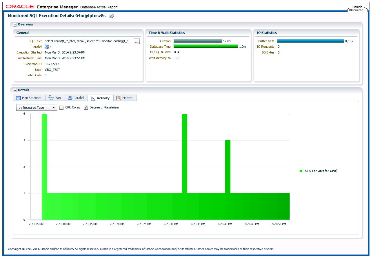
Compare this activity pattern to the one shown in the first part of the series. Also note how the Database Time is still approximately 60 seconds, so this execution hasn’t really spent more time in the database than before, but the uneven distribution of work leads to the longer overall execution time, since it has to wait for the Parallel Execution Server to complete that has to do the majority of work.
Before we discuss options for how we can address Parallel Execution Skew and look at more scenarios where we might encounter it, we’ll explore in the next part of this series a new feature of Oracle 12c that – for the time being in a limited number of scenarios – allows Oracle to address the skew problem automatically.
Load comments