Clustering is a type of unsupervised machine learning that involves identifying groups within data, where each of the data points within the groups is similar (or related) and different (or unrelated) to data points in other groups. The greater the similarity (or homogeneity) within a group and the more significant the difference between groups, the better or more distinct the clustering. Some clustering applications are recommendation engines, social network analysis, population segmentation, etc. This article explains how to use clustered data to gain insights.

The need for clustering

The value of clustering comes from its ability to quickly give insights from large unstructured data and organize the data into subsets which can be used to drive actions. Data practitioners don’t always have the luxury of having well-labeled datasets. Because clustering is usually a first step to get some insights from the data, by running a clustering algorithm it’s possible to label a large dataset without manual intervention.

What are the types of clustering algorithms?

• K-Means –a clustering algorithm used across various domains such as customer segmentation, and fraud detection. The algorithm segregates a dataset into multiple groups, which are also known as clusters. Data points are assigned to clusters based on Euclidian Distance. A caveat with using K-Means is having to pre-define the number of clusters at the time of running the algorithm. There are methods such as scree plot to identify the optimal number of clusters to define.
• Hierarchical Agglomerative clustering –a connectivity-based clustering approach where the algorithm groups similar objects into clusters. The end result will be various clusters that are distinct from one another, and the objects within each cluster are broadly like each other. It’s a bottom-up approach; each observation starts as its own cluster, and pairs of clusters are merged as one moves up the hierarchy.
• Density Based Clustering (DBSCAN)–a commonly used approach to cluster high density regions. It is based on the notion of clusters and noise. The main consideration here is that for each object in a cluster, the neighborhood of that object within a certain radius contains a minimum number of points. However, it has a limitation when dealing with clusters of varying densities or high dimensional data. To overcome this limitation, HDBSCAN is proposed which is a variant of DBSCAN that allows varying density clusters.

What type of distance function to use in clustering algorithms?

A distance function provides the distance between data points that need to be clustered. Below are a few types of distance functions that can be used with clustering algorithms:

• Minkowski Distance – calculates the distance between two real-valued vectors
• Manhattan Distance – the distance between two points measured along axes at right angles.
• Euclidean Distance – the length of a line segment between two data points

What are some challenges with clustering models?

• Outliers – Having outliers within your dataset can result in non-optimal clustering results as it affects the distance calculations during cluster formation.
• Sparse Data – If your dataset has dimensions with mostly 0s or NAs, this can affect the distance calculation as well as computational efficiency issues.
• Large number of records – if your dataset has a large number of records, this can lead to computation efficiency issues. Most clustering algorithms do not scale linearly with increasing sample size and/or dimensions.
• Curse of dimensionality – if the number of dimensions in your dataset is high, it could lead to sub-optimal performance and increase computation time and cost. One solution for this issue is to use principal component analysis.

How to handle categorical and continuous data while clustering?

Datasets are sometimes a mix of numerical and categorical data. There are a couple of ways to handle categorical data such as one-hot encoding, but this could increase the number of dimensions in your dataset. Hence, one could use Gower distance which is a metric that can be used to calculate the distance between objects whose features are of mix datatypes such as categorical and quantitative. This distance is scaled in a range of 0 to 1, with 0 being similar and 1 being different.

When the distribution of continuous variables I skewed with a varying range of values, directly using these features can cause adverse effects in clustering. Hence, these features can be quantized using fixed-width binning.

Is normalizing the dataset required for clustering?

In clustering, the distance between data points is calculated to cluster close data points together. The data is normalized to make sure all dimensions are given similar weight. This helps to prevent features with large numerical values from dominating in distance functions. There are multiple ways of normalization such as min-max normalization, z-score normalization, etc.

Implementation of Density Based Scan (DBSCAN) on transactional data

This example will implement the DBSCAN algorithm on a dataset provided by sklearn. It uses the following python packages:

• Pandas – an open-source data analysis and manipulation tool
• Sklearn – Simple and efficient tools for predictive data analysis
• Seaborn – a Python based package for plotting interactive visualizations

To install any of the above packages, execute pip install package_name within a terminal window.

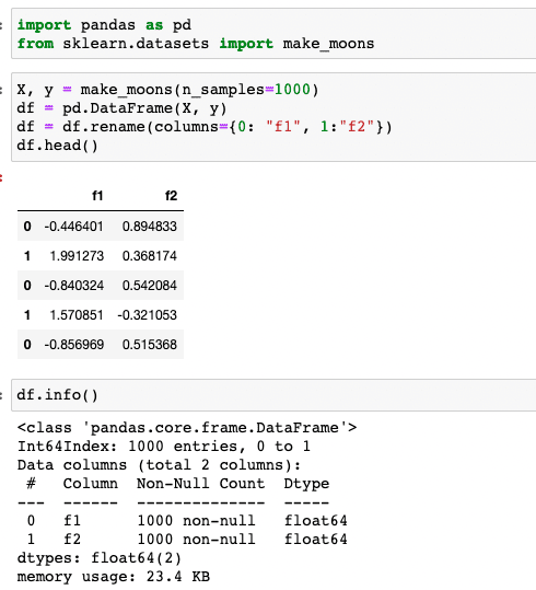
Step 1: Load data into pandas. There are 1000 records with 2 features

The above code reads a dataset to be clustered into a pandas dataframe and displays first the 5 records using the .head() function. The .info() function displays metadata of the variables in the dataset such as datatype and number of records

Step 2: Implementing DBSCAN algorithm with default settings to the dataset

In this piece of code, the DBSCAN package is imported from the sklearn library and applied onto the dataset. The labels column will contain the cluster ID of the data points.

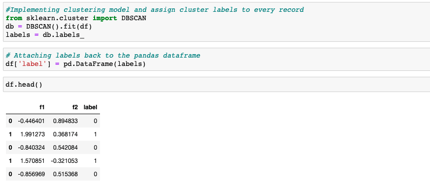
As you can see, the data points are segregated into two different categories 0 and 1.

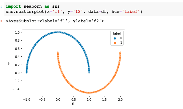
Step 3: Visualize the clusters

You can finally visualize the clustered results using a scatter plot from the seaborn library. As you can see form the plot, the datapoints are clearly segregated in two different clusters.

Metrics to evaluate the performance of a clustering model

There are multiple ways to measure the clustering results based on the problem that is trying to be solved. While measures like Silhouette Coefficient give a sense of how well apart clusters from each other are, it may or may not tell how good the clusters for your business problem are. Hence, one way is to generate cluster level metrics by aggregating data points within every cluster and intuitively marking clusters as useful or not, the other way can be sampling data points from every cluster and manually auditing them for usefulness.

References

https://developers.google.com/machine-learning/clustering/clustering-algorithms

https://scikit-learn.org/stable/modules/generated/sklearn.cluster.DBSCAN.html

https://scikit-learn.org/stable/modules/generated/sklearn.datasets.make_moons.html